Data Structure for self Learning

 

Data Structure - Recursion Basics

Some computer programming languages allow a module or function to call itself. This technique is known as recursion. In recursion, a function α either calls itself directly or calls a function β that in turn calls the original function α. The function α is called recursive function.

in Python Recursion work upto (1000 by Default)

Example − a function calling itself.

int function(int value) {
   if(value < 1)
      return;
   function(value - 1);

   printf("%d ",value);   
}

Example − a function that calls another function which in turn calls it again.

int function1(int value1) {
   if(value1 < 1)
      return;
   function2(value1 - 1);
   printf("%d ",value1);   
}
int function2(int value2) {
   function1(value2);
}

Properties

A recursive function can go infinite like a loop. To avoid infinite running of recursive function, there are two properties that a recursive function must have −

• Base criteria − There must be at least one base criteria or condition, such that, when this condition is met the function stops calling itself recursively.

• Progressive approach − The recursive calls should progress in such a way that each time a recursive call is made it comes closer to the base criteria.

Implementation

Many programming languages implement recursion by means of stacks. Generally, whenever a function (caller) calls another function (callee) or itself as callee, the caller function transfers execution control to the callee. This transfer process may also involve some data to be passed from the caller to the callee.

This implies, the caller function has to suspend its execution temporarily and resume later when the execution control returns from the callee function. Here, the caller function needs to start exactly from the point of execution where it puts itself on hold. It also needs the exact same data values it was working on. For this purpose, an activation record (or stack frame) is created for the caller function.

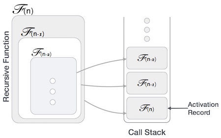
This activation record keeps the information about local variables, formal parameters, return address and all information passed to the caller function.

Blog link:-https://www.tutorialspoint.com/data_structures_algorithms/recursion_basics.htm#:~:text=Some%20computer%20programming%20languages%20allow,calls%20the%20original%20function%20%CE%B1.

Fibonacci is best example of Recursion

def get_fib(position):

    if position == 0 or position == 1:

        return position

    return get_fib(position - 1) + get_fib(position - 2)

print (get_fib(1))

print (get_fib(9))

print (get_fib(11))

print (get_fib(0))

output:-

1

34

89

0

Data Structure - Sorting Techniques

Sorting refers to arranging data in a particular format. Sorting algorithm specifies the way to arrange data in a particular order. Most common orders are in numerical or lexicographical order.

Stable and Not Stable Sorting

If a sorting algorithm, after sorting the contents, does not change the sequence of similar content in which they appear, it is called stable sorting.

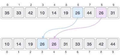
If a sorting algorithm, after sorting the contents, changes the sequence of similar content in which they appear, it is called unstable sorting.

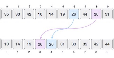
Stability of an algorithm matters when we wish to maintain the sequence of original elements, like in a tuple for example.

Blog Link:-https://www.tutorialspoint.com/data_structures_algorithms/sorting_algorithms.htm#:~:text=Sorting%20refers%20to%20arranging%20data,in%20numerical%20or%20lexicographical%20order.

Data Structure - Bubble Sort Algorithm

Bubble sort is a simple sorting algorithm. This sorting algorithm is comparison-based algorithm in which each pair of adjacent elements is compared and the elements are swapped if they are not in order. This algorithm is not suitable for large data sets as its average and worst case complexity are of Ο(n2) where n is the number of items.

How Bubble Sort Works?

We take an unsorted array for our example. Bubble sort takes Ο(n2) time so we're keeping it short and precise.

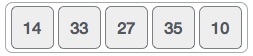
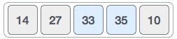
Bubble sort starts with very first two elements, comparing them to check which one is greater.

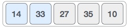
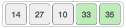
In this case, value 33 is greater than 14, so it is already in sorted locations. Next, we compare 33 with 27.

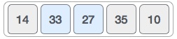
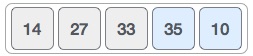
We find that 27 is smaller than 33 and these two values must be swapped.

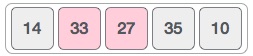
The new array should look like this −

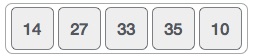
Next we compare 33 and 35. We find that both are in already sorted positions.

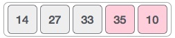
Then we move to the next two values, 35 and 10.

We know then that 10 is smaller 35. Hence they are not sorted.

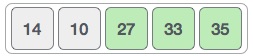
We swap these values. We find that we have reached the end of the array. After one iteration, the array should look like this −

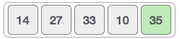
To be precise, we are now showing how an array should look like after each iteration. After the second iteration, it should look like this −

Notice that after each iteration, at least one value moves at the end.

And when there's no swap required, bubble sorts learns that an array is completely sorted.

Now we should look into some practical aspects of bubble sort.

Algorithm

We assume list is an array of n elements. We further assume that swap function swaps the values of the given array elements.

begin BubbleSort(list)

   for all elements of list
      if list[i] > list[i+1]
         swap(list[i], list[i+1])
      end if
   end for
   
   return list
   
end BubbleSort

Pseudocode

We observe in algorithm that Bubble Sort compares each pair of array element unless the whole array is completely sorted in an ascending order. This may cause a few complexity issues like what if the array needs no more swapping as all the elements are already ascending.

To ease-out the issue, we use one flag variable swapped which will help us see if any swap has happened or not. If no swap has occurred, i.e. the array requires no more processing to be sorted, it will come out of the loop.

Pseudocode of BubbleSort algorithm can be written as follows −

procedure bubbleSort( list : array of items )

   loop = list.count;
   
   for i = 0 to loop-1 do:
      swapped = false
		
      for j = 0 to loop-1 do:
      
         /* compare the adjacent elements */   
         if list[j] > list[j+1] then
            /* swap them */
            swap( list[j], list[j+1] )		 
            swapped = true
         end if
         
      end for
      
      /*if no number was swapped that means 
      array is sorted now, break the loop.*/
      
      if(not swapped) then
         break
      end if
      
   end for
   
end procedure return list

Implementation

One more issue we did not address in our original algorithm and its improvised pseudocode, is that, after every iteration the highest values settles down at the end of the array. Hence, the next iteration need not include already sorted elements. For this purpose, in our implementation, we restrict the inner loop to avoid already sorted values.

Data Structures - Merge Sort Algorithm

Merge sort is a sorting technique based on divide and conquer technique. With worst-case time complexity being Ο(n log n), it is one of the most respected algorithms.

Merge sort first divides the array into equal halves and then combines them in a sorted manner.

Algorithm

Merge sort keeps on dividing the list into equal halves until it can no more be divided. By definition, if it is only one element in the list, it is sorted. Then, merge sort combines the smaller sorted lists keeping the new list sorted too.

Step 1 − if it is only one element in the list it is already sorted, return.
Step 2 − divide the list recursively into two halves until it can no more be divided.
Step 3 − merge the smaller lists into new list in sorted order.

blogLink:-https://www.tutorialspoint.com/data_structures_algorithms/merge_sort_algorithm.htm#:~:text=Merge%20sort%20is%20a%20sorting,them%20in%20a%20sorted%20manner.

blog2Link:- https://algs4.cs.princeton.edu/22mergesort/

Data Structure and Algorithms - Quick Sort

Quick sort is a highly efficient sorting algorithm and is based on partitioning of array of data into smaller arrays. A large array is partitioned into two arrays one of which holds values smaller than the specified value, say pivot, based on which the partition is made and another array holds values greater than the pivot value.

Quicksort partitions an array and then calls itself recursively twice to sort the two resulting subarrays. This algorithm is quite efficient for large-sized data sets as its average and worst-case complexity are O(nLogn) and image.png(n2), respectively.

Partition in Quick Sort

Following animated representation explains how to find the pivot value in an array.

The pivot value divides the list into two parts. And recursively, we find the pivot for each sub-lists until all lists contains only one element.

Quick Sort Pivot Algorithm

Based on our understanding of partitioning in quick sort, we will now try to write an algorithm for it, which is as follows.

Step 1 − Choose the highest index value has pivot
Step 2 − Take two variables to point left and right of the list excluding pivot
Step 3 − left points to the low index
Step 4 − right points to the high
Step 5 − while value at left is less than pivot move right
Step 6 − while value at right is greater than pivot move left
Step 7 − if both step 5 and step 6 does not match swap left and right
Step 8 − if left ≥ right, the point where they met is new pivot

Quick Sort Pivot Pseudocode

The pseudocode for the above algorithm can be derived as −

function partitionFunc(left, right, pivot)
   leftPointer = left
   rightPointer = right - 1

   while True do
      while A[++leftPointer] < pivot do
         //do-nothing            
      end while
		
      while rightPointer > 0 && A[--rightPointer] > pivot do
         //do-nothing         
      end while
		
      if leftPointer >= rightPointer
         break
      else                
         swap leftPointer,rightPointer
      end if
		
   end while 
	
   swap leftPointer,right
   return leftPointer
	
end function

Quick Sort Algorithm

Using pivot algorithm recursively, we end up with smaller possible partitions. Each partition is then processed for quick sort. We define recursive algorithm for quicksort as follows −

Step 1 − Make the right-most index value pivot
Step 2 − partition the array using pivot value
Step 3 − quicksort left partition recursively
Step 4 − quicksort right partition recursively

Quick Sort Pseudocode

To get more into it, let see the pseudocode for quick sort algorithm −

procedure quickSort(left, right)

   if right-left <= 0
      return
   else     
      pivot = A[right]
      partition = partitionFunc(left, right, pivot)
      quickSort(left,partition-1)
      quickSort(partition+1,right)    
   end if		
   
end procedure

blogLink:-https://www.tutorialspoint.com/data_structures_algorithms/quick_sort_algorithm.htm#:~:text=Quick%20sort%20is%20a%20highly,of%20data%20into%20smaller%20arrays.&text=Quicksort%20partitions%20an%20array%20and,sort%20the%20two%20resulting%20subarrays.

Code:-

def partition(arr, low, high):

    i = (low-1)      # index of smaller element

    pivot = arr[high]    # pivot

    for j in range(low, high):

        # If current element is smaller than or

        # equal to pivot

        if arr[j] <= pivot:

            # increment index of smaller element

            i = i+1

            arr[i], arr[j] = arr[j], arr[i]

    arr[i+1], arr[high] = arr[high], arr[i+1]

    return (i+1)

# The main function that implements QuickSort

# arr[] --> Array to be sorted,

# low --> Starting index,

# high --> Ending index

# Function to do Quick sort

def quickSort(arr, low, high):

    if len(arr) == 1:

        return arr

    if low < high:

        # pi is partitioning index, arr[p] is now

        # at right place

        pi = partition(arr, low, high)

        # Separately sort elements before

        # partition and after partition

        quickSort(arr, low, pi-1)

        quickSort(arr, pi+1, high)

# Driver code to test above

arr = [10, 7, 8, 9, 1, 5]

n = len(arr)

quickSort(arr, 0, n-1)

print("Sorted array is:")

for i in range(n):

    print(arr[i] , end = " ")

Output:-

[1, 3, 4, 6, 9, 14, 20, 21, 21, 25]